Multistart Optimization with ParmEst - Pyomo.DoE Workshop and Tutorials

Parameter estimation problems are often nonconvex, meaning that the objective function $g(\boldsymbol{x}, \boldsymbol{y};\boldsymbol{\theta})$ may contain multiple local minima. As a result, the solution obtained by a nonlinear optimization solver can depend strongly on the initial guess for $\boldsymbol{\theta}$ .

Multistart optimization is a practical strategy to address this challenge. Instead of solving the problem once from a single initial point, we solve it multiple times from different initializations and compare the resulting solutions.

This approach helps:

Increase the likelihood of identifying a global or near-global optimum
Assess the robustness of parameter estimates
Explore the structure of the objective landscape

Import the Necessary Packages¶

import sys
import logging
import pandas as pd
import numpy as np

# If running on Google Colab, install Pyomo and Ipopt via IDAES
on_colab = "google.colab" in sys.modules
if on_colab:
    !wget "https://raw.githubusercontent.com/dowlinglab/pyomo-doe/main/notebooks/tclab_pyomo.py"

# import TCLab model, simulation, and data analysis functions
from tclab_pyomo import (
    TC_Lab_data,
    TC_Lab_experiment,
    extract_multistart_sampling,
    plot_profile_likelihood,
)

# set default number of states in the TCLab model
number_tclab_states = 2

Load the Experimental Data¶

# load experimental data
if on_colab:
    file = "https://raw.githubusercontent.com/dowlinglab/pyomo-doe/main/data/tclab_sine_test_5min_period.csv"
else:
    file = "../data/tclab_sine_test_5min_period.csv"
df = pd.read_csv(file)

# store in custom data class
tc_data = TC_Lab_data(
    name="Sine Wave Test for Heater 1",
    time=df["Time"].values,
    T1=df["T1"].values,
    u1=df["Q1"].values,
    P1=200,
    TS1_data=None,
    T2=df["T2"].values,
    u2=df["Q2"].values,
    P2=200,
    TS2_data=None,
    Tamb=df["T1"].values[0],
)

# set default number of states in the TCLab model
number_tclab_states = 2

Multistart in ParmEst¶

The multistart functionality in ParmEst automates this process by generating multiple initial guesses for $\boldsymbol{\theta}$ within user-defined bounds and solving the parameter estimation problem repeatedly.

Initial points are sampled between predefined lower and upper bounds using one of the following methods:

Uniform random sampling
Latin hypercube sampling (LHS)
Sobol sequence sampling

Each sampled point defines a new initialization of $\boldsymbol{\theta}$ , and the optimization
problem is solved independently for each case.

TC Lab Parameter Estimation Problem Statement¶

As stated previously:

We seek to estimate the heat transfer parameters, $C_p^H$ , $C_p^S$ , $U_a$ , and $U_b$ from the sensor temperature data outlined above.

The predictions of the sensor temperature are obtained from the following model structure:

\begin{align*} C_p^H \frac{dT_H}{dt} & = U_a (T_{amb} - T_H) + U_c (T_S - T_H) + \alpha P u(t)\\ C_p^S \frac{dT_S}{dt} & = - U_b (T_S - T_H) \end{align*}

(1)

\begin{align*} \text{control input data}\qquad u(t_i) & = \bar{u}_{i}, \forall i \in \mathcal{T} \\ \text{initial condition}\qquad T_H(t_0) & = T_{amb} \\ \text{initial condition}\qquad T_S(t_0) & = T_{amb} \end{align*}

(2)

where $T_{H}$ and $T_{S}$ are the heater and sensor temperatures in $^{\circ} \text{C}$ , respectively, $T_{amb}$ is the ambient temperature in $^{\circ} \text{C}$ , $C_p^H$ and $C_p^S$ are the heat capacity of the heater and sensor in $\text{J}/^{\circ} \text{C}$ , respectively, $U_{a}$ and $U_{b}$ are the heat transfer coefficients from the heater to the sensor and the sensor to ambient (in $\text{W}/^{\circ} \text{C}$ ), respectively, $P$ is the maximum power limit in $\text{bit}$ , $u$ is the heater power in $\%$ , and $\alpha$ is constant that converts the unit of $P u(t)$ into $\text{W}$ .

The difference here is we are using sampling techniques to automate the process of searching from multiple initial values of the estimated heat transfer parameters.

# # Import parmest
import pyomo.contrib.parmest.parmest as parmest

# Set logging level to ERROR to suppress solver output and warnings from parmest
logging.basicConfig(level=logging.ERROR, force=True)

parmest_logger = logging.getLogger("pyomo.contrib.parmest.parmest")
parmest_logger.setLevel(logging.ERROR)

# First, we define an Experiment object within parmest
TC_Lab_sine_exp = TC_Lab_experiment(data=tc_data, number_of_states=number_tclab_states)

solver_options = {"linear_solver": "ma57", "max_iter": 1000}


# Set some common options for all multistart estimation runs
common_multistart_options = {"n_restarts": 15, "seed": 532, "save_results": False}

# Since everything has been labeled properly in the Experiment object, we simply invoke
# parmest's Estimator function to estimate the parameters.
pest_uniform = parmest.Estimator(
    [TC_Lab_sine_exp], obj_function="SSE", tee=True, solver_options=solver_options
)

results_df, best_theta_uniform, best_obj_uniform = pest_uniform.theta_est_multistart(
    multistart_sampling_method="uniform_random",
    n_restarts=common_multistart_options["n_restarts"],
    seed=common_multistart_options["seed"],
    save_results=common_multistart_options["save_results"],
)

Fetching long content....

Let’s see how to access the regression results:

print("Estimated parameters:\n", best_theta_uniform)
print("Best objective function value:", best_obj_uniform)

Estimated parameters:
 {'Ua': 0.041705173357635135, 'Ub': 0.017064930852255578, 'inv_CpH': 0.1707011238132523, 'inv_CpS': 3.137848009988043}
Best objective function value: 53.773992845808294

# Sort the results in ascending order of objective function value to identify the best runs
results_df_sorted = results_df.sort_values(
    by="final objective", ascending=True
).reset_index(drop=True)
print("\nTop 5 multistart runs based on final objective function value:")
results_df_sorted[
    [
        "converged_Ua",
        "converged_Ub",
        "converged_inv_CpH",
        "converged_inv_CpS",
        "final objective",
    ]
].head()


Top 5 multistart runs based on final objective function value:

Compare Different Multistart Sampling Methods¶

# latin hypercube sampling
pest_lhs = parmest.Estimator(
    [TC_Lab_sine_exp], obj_function="SSE", tee=False, solver_options=solver_options
)

results_df_lhs, best_theta_lhs, best_obj_lhs = pest_lhs.theta_est_multistart(
    multistart_sampling_method="latin_hypercube",
    n_restarts=common_multistart_options["n_restarts"],
    seed=common_multistart_options["seed"],
    save_results=common_multistart_options["save_results"],
)

# Sobol sampling
pest_sobol = parmest.Estimator(
    [TC_Lab_sine_exp], obj_function="SSE", tee=False, solver_options=solver_options
)

results_df_sobol, best_theta_sobol, best_obj_sobol = pest_sobol.theta_est_multistart(
    multistart_sampling_method="sobol_sampling",
    n_restarts=common_multistart_options["n_restarts"],
    seed=common_multistart_options["seed"],
    save_results=common_multistart_options["save_results"],
)

theta_values_df = pd.DataFrame(
    {
        "random_uniform": best_theta_uniform,
        "latin_hypercube": best_theta_lhs,
        "sobol_sampling": best_theta_sobol,
    }
)
print(
    "\nBest estimated parameters for different multistart sampling methods:\n",
    theta_values_df,
)

# Best objective function values for different multistart sampling methods
obj_values_df = pd.DataFrame(
    {
        "random_uniform": best_obj_uniform,
        "latin_hypercube": best_obj_lhs,
        "sobol_sampling": best_obj_sobol,
    },
    index=["Best Objective Value"],
)
print(
    "\nBest objective function values for different multistart sampling methods:\n",
    obj_values_df,
)


Best estimated parameters for different multistart sampling methods:
          random_uniform  latin_hypercube  sobol_sampling
Ua             0.041705         0.041705        0.041705
Ub             0.017065         0.017199        0.017104
inv_CpH        0.170701         0.170791        0.170727
inv_CpS        3.137848         3.111786        3.130236

Best objective function values for different multistart sampling methods:
                       random_uniform  latin_hypercube  sobol_sampling
Best Objective Value       53.773993        53.773993       53.773993

# Round the best objective function values to 4 decimal places for easier comparison

results_df["final objective"] = results_df["final objective"].round(6)
results_df_lhs["final objective"] = results_df_lhs["final objective"].round(6)
results_df_sobol["final objective"] = results_df_sobol["final objective"].round(6)


# Compare the number of unique local minima found by different multistart sampling methods

num_unique_minima_uniform = len(results_df["final objective"].unique())
num_unique_minima_lhs = len(results_df_lhs["final objective"].unique())
num_unique_minima_sobol = len(results_df_sobol["final objective"].unique())

print("\nNumber of unique local minima found by different multistart sampling methods:")
print(f"Random Uniform Sampling: {num_unique_minima_uniform}")
print(f"Latin Hypercube Sampling: {num_unique_minima_lhs}")
print(f"Sobol Sampling: {num_unique_minima_sobol}")


Number of unique local minima found by different multistart sampling methods:
Random Uniform Sampling: 1
Latin Hypercube Sampling: 1
Sobol Sampling: 2

# Plot starting theta values for different multistart sampling methods
fig, axes = extract_multistart_sampling(results_df, results_df_lhs, results_df_sobol)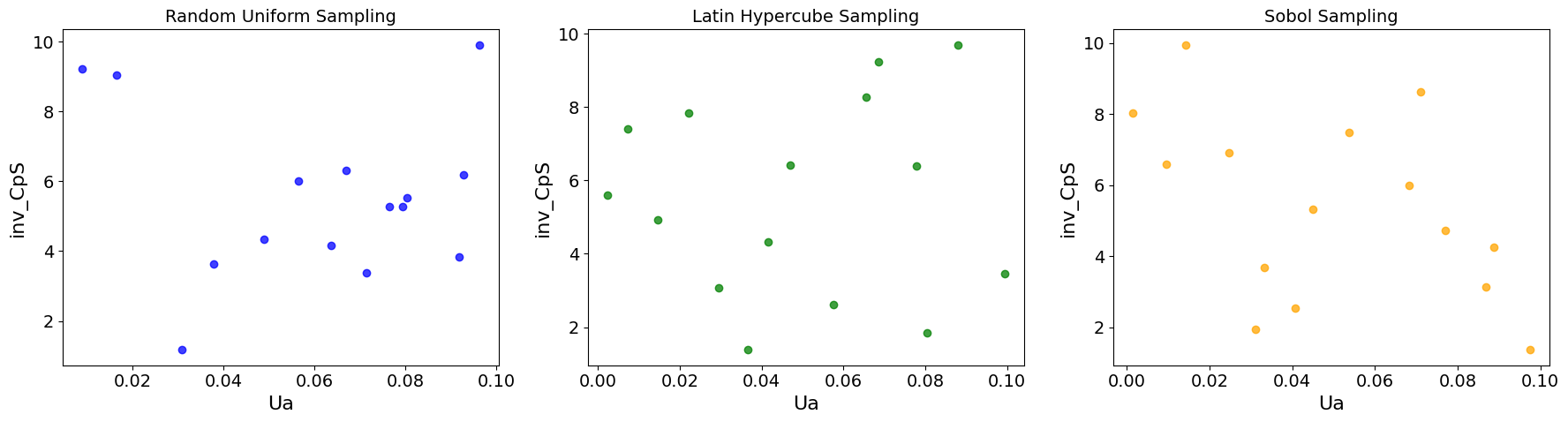

Takeaways from the Multistart Optimization Results¶

The different methods converge to different estimates, but the same objective value
Differences in the parameters with same objective value points to a potential identifiability problem.
Stratified sampling techniques (LHS and Sobol) cover more area of the sample space
Random uniform sampling, as shown above, can sample multiple points in same region.