Getting Started: Parameter Estimation Basics - Pyomo.DoE Workshop and Tutorials

The goal of parameter estimation is to estimate values for a vector, $\boldsymbol{\theta}$ , from experimental data (observations) to use in the functional form:

\boldsymbol{y}_i = \boldsymbol{f}\left(\boldsymbol{x}_{i}, \boldsymbol{\theta}\right) + \boldsymbol{\varepsilon}_i \quad \forall \; i \in \{1, \ldots, n\}

(1)

where $\boldsymbol{y}_{i} \in \mathbb{R}^m$ are observations of the measured or output variables, $\boldsymbol{f(\cdot)}$ is the model function, $\boldsymbol{x}_{i} \in \mathbb{R}^{q}$ are the decision or input variables, $\boldsymbol{\theta} \in \mathbb{R}^p$ are the model parameters, $\boldsymbol{\varepsilon}_{i} \in \mathbb{R}^m$ are the measurement errors, and $n$ is the number of experiments.

The following least squares objective can be used to estimate parameter values assuming that the measurement errors follow a Gaussian distribution:

\min_{\boldsymbol{\theta}} \, g(\boldsymbol{x}, \boldsymbol{y};\boldsymbol{\theta})

(2)

where $g(\boldsymbol{x}, \boldsymbol{y};\boldsymbol{\theta})$ can be:

$\textbf{Sum of squared errors}$
If the measurement errors (which are assumed to follow a Gaussian distribution) are independent and identically distributed, the objective function can be defined as the sum of squared errors

g(\boldsymbol{x}, \boldsymbol{y};\boldsymbol{\theta}) = \sum_{i = 1}^{n} \left(\boldsymbol{y}_{i} - \boldsymbol{f}(\boldsymbol{x}_{i};\boldsymbol{\theta}) \right)^\text{T} \left(\boldsymbol{y}_{i} - \boldsymbol{f}(\boldsymbol{x}_{i};\boldsymbol{\theta})\right)

(3)

$\textbf{Weighted sum of squared errors}$
When the measurement errors are correlated and their covariance matrix, $\boldsymbol{\Sigma}_{\boldsymbol{y}}$ , is known a priori, the objective function is defined as the weighted sum of squared errors

g(\boldsymbol{x}, \boldsymbol{y};\boldsymbol{\theta}) = \frac{1}{2} \sum_{i = 1}^{n} \left(\boldsymbol{y}_{i} - \boldsymbol{f}(\boldsymbol{x}_{i};\boldsymbol{\theta}) \right)^\text{T} \boldsymbol{\Sigma}_{\boldsymbol{y}}^{-1} \left(\boldsymbol{y}_{i} - \boldsymbol{f}(\boldsymbol{x}_{i};\boldsymbol{\theta})\right)

(4)

Custom objectives can also be defined for parameter estimation.

In the applications of interest to us, the function $g(\cdot)$ is usually defined as an optimization problem with a large number of (perhaps constrained) optimization variables, a subset of which are fixed at values $\boldsymbol{x}$ when the optimization is performed. In other applications, the values of $\boldsymbol{\theta}$ are fixed parameter values, but for the problem formulation above, the values of $\boldsymbol{\theta}$ are the primary optimization variables. Note that in general, the function $g(\cdot)$ will have a large set of parameters that are not included in $\boldsymbol{\theta}$ .

Import the Necessary Packages¶

import sys

# If running on Google Colab, install Pyomo and Ipopt via IDAES
on_colab = "google.colab" in sys.modules
if on_colab:
    !wget "https://raw.githubusercontent.com/dowlinglab/pyomo-doe/main/notebooks/tclab_pyomo.py"

# import TCLab model, simulation, and data analysis functions
from tclab_pyomo import (
    TC_Lab_data,
    TC_Lab_experiment,
    extract_results,
    extract_plot_results,
)

# set default number of states in the TCLab model
number_tclab_states = 2

Load and Explore the Experimental Data¶

import pandas as pd

if on_colab:
    file = "https://raw.githubusercontent.com/dowlinglab/pyomo-doe/main/data/tclab_sine_test_5min_period.csv"
else:
    file = "../data/tclab_sine_test_5min_period.csv"
df = pd.read_csv(file)
df[["Time", "T1", "Q1", "Q2"]].head()  # the Q2 column entries are 0 because
# we are considering the two-state model

ax = df.plot(x="Time", y=["T1"], xlabel="Time (s)", ylabel="Temperature (°C)")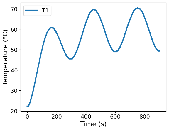

ax = df.plot(x="Time", y=["Q1", "Q2"], xlabel="Time (s)", ylabel="Heater Power (%)")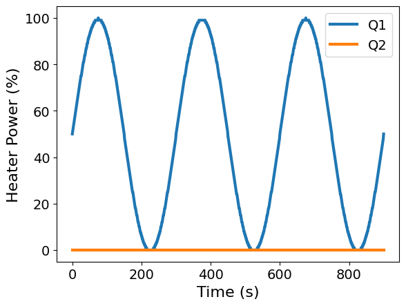

Store in Custom Data Class¶

In the file tclab_pyomo.py, we defined a dataclass for convenience. It is essentially a light weight container to store experimental data.

tc_data = TC_Lab_data(
    name="Sine Wave Test for Heater 1",
    time=df["Time"].values,
    T1=df["T1"].values,
    u1=df["Q1"].values,
    P1=200,
    TS1_data=None,
    T2=df["T2"].values,
    u2=df["Q2"].values,
    P2=200,
    TS2_data=None,
    Tamb=df["T1"].values[0],
)

tc_data.to_data_frame().iloc[:, :4].head()

TC Lab Parameter Estimation Problem Statement¶

We seek to estimate the heat transfer parameters, $C_p^H$ , $C_p^S$ , $U_a$ , and $U_b$ from the sensor temperature data outlined above.

The predictions of the sensor temperature are obtained from the following model structure:

\begin{align*} C_p^H \frac{dT_H}{dt} & = U_a (T_{amb} - T_H) + U_c (T_S - T_H) + \alpha P u(t)\\ C_p^S \frac{dT_S}{dt} & = - U_b (T_S - T_H) \end{align*}

(5)

\begin{align*} \text{control input data}\qquad u(t_i) & = \bar{u}_{i}, \forall i \in \mathcal{T} \\ \text{initial condition}\qquad T_H(t_0) & = T_{amb} \\ \text{initial condition}\qquad T_S(t_0) & = T_{amb} \end{align*}

(6)

where $T_{H}$ and $T_{S}$ are the heater and sensor temperatures in $^{\circ} \text{C}$ , respectively, $T_{amb}$ is the ambient temperature in $^{\circ} \text{C}$ , $C_p^H$ and $C_p^S$ are the heat capacity of the heater and sensor in $\text{J}/^{\circ} \text{C}$ , respectively, $U_{a}$ and $U_{b}$ are the heat transfer coefficients from the heater to the sensor and the sensor to ambient (in $\text{W}/^{\circ} \text{C}$ ), respectively, $P$ is the maximum power limit in $\text{bit}$ , $u$ is the heater power in $\%$ , and $\alpha$ is constant that converts the unit of $P u(t)$ into $\text{W}$ .

In the tclab_pyomo.py model, we defined several helper functions:

extract_results takes a Pyomo model and returns the results stored in an instance of the TC_Lab_data dataclass.
extract_plot_results takes experimental data (stored in a TC_Lab_data instance) and a Pyomo model. The function then generates plots showing the data and model predictions.
results_summary summarizes the Pyomo.DoE results. We’ll use this later in the workshop.

Parameter Estimation with ParmEst¶

In ParmEst, the TC Lab parameter estimation problem can be solved using two objective functions as mentioned in the introduction of this page:

Sum of squared errors (SSE)
Weighted sum of squared errors (WSSE)

Custom objectives may also be constructed and used to estimate the model parameters; however, uncertainty quantification for such objective is not supported.

Import ParmEst¶

import pyomo.contrib.parmest.parmest as parmest

Create a TC Lab Experiment Object¶

# define an Experiment object within ParmEst
TC_Lab_sine_exp = TC_Lab_experiment(data=tc_data, number_of_states=number_tclab_states)

Estimate the Parameters using the SSE Objective¶

Since everything has been labeled properly in the Experiment object, we simply invoke ParmEst’s Estimator function to estimate the parameters using the SSE objective.

pest_SSE = parmest.Estimator([TC_Lab_sine_exp], obj_function="SSE", tee=True)

obj_SSE, theta_SSE = pest_SSE.theta_est()

Ipopt 3.13.2: 

******************************************************************************
This program contains Ipopt, a library for large-scale nonlinear optimization.
 Ipopt is released as open source code under the Eclipse Public License (EPL).
         For more information visit http://projects.coin-or.org/Ipopt

This version of Ipopt was compiled from source code available at
    https://github.com/IDAES/Ipopt as part of the Institute for the Design of
    Advanced Energy Systems Process Systems Engineering Framework (IDAES PSE
    Framework) Copyright (c) 2018-2019. See https://github.com/IDAES/idaes-pse.

This version of Ipopt was compiled using HSL, a collection of Fortran codes
    for large-scale scientific computation.  All technical papers, sales and
    publicity material resulting from use of the HSL codes within IPOPT must
    contain the following acknowledgement:
        HSL, a collection of Fortran codes for large-scale scientific
        computation. See http://www.hsl.rl.ac.uk.
******************************************************************************

This is Ipopt version 3.13.2, running with linear solver ma27.

Number of nonzeros in equality constraint Jacobian...:    15301
Number of nonzeros in inequality constraint Jacobian.:        0
Number of nonzeros in Lagrangian Hessian.............:     7203

Total number of variables............................:     3606
                     variables with only lower bounds:        0
                variables with lower and upper bounds:     1804
                     variables with only upper bounds:        0
Total number of equality constraints.................:     3602
Total number of inequality constraints...............:        0
        inequality constraints with only lower bounds:        0
   inequality constraints with lower and upper bounds:        0
        inequality constraints with only upper bounds:        0

iter    objective    inf_pr   inf_du lg(mu)  ||d||  lg(rg) alpha_du alpha_pr  ls
   0  4.7112445e+04 3.12e-01 1.14e+01  -1.0 0.00e+00    -  0.00e+00 0.00e+00   0
   1  1.6610939e+02 3.56e-02 1.91e+04  -1.0 9.61e+00    -  6.00e-01 1.00e+00f  1
   2  1.6937122e+02 8.45e-03 8.59e+03  -1.0 9.46e-01   2.0 9.93e-01 8.97e-01h  1
   3  5.5361730e+01 3.56e-04 1.76e+03  -1.0 5.21e-01    -  1.00e+00 1.00e+00f  1
   4  5.3777130e+01 1.29e-04 6.07e+01  -1.0 1.36e-01    -  9.85e-01 1.00e+00f  1
   5  5.3780334e+01 1.22e-02 5.99e+00  -1.0 9.89e-01    -  1.00e+00 1.00e+00f  1
   6  5.3779789e+01 2.06e-02 4.92e-01  -1.0 9.92e-01    -  1.00e+00 1.00e+00h  1
   7  5.3772236e+01 3.48e-04 1.52e-01  -1.7 9.55e-02    -  1.00e+00 1.00e+00h  1
   8  5.3774001e+01 2.94e-05 3.90e-03  -2.5 3.32e-02    -  1.00e+00 1.00e+00h  1
   9  5.3773993e+01 2.54e-06 3.88e-04  -3.8 9.06e-03    -  1.00e+00 1.00e+00h  1
iter    objective    inf_pr   inf_du lg(mu)  ||d||  lg(rg) alpha_du alpha_pr  ls
  10  5.3773993e+01 1.24e-07 4.72e-06  -5.7 2.01e-03    -  1.00e+00 1.00e+00h  1
  11  5.3773993e+01 1.49e-09 6.46e-09  -8.6 2.21e-04    -  1.00e+00 1.00e+00h  1

Number of Iterations....: 11

                                   (scaled)                 (unscaled)
Objective...............:   5.3773992845814796e+01    5.3773992845814796e+01
Dual infeasibility......:   6.4556607083697884e-09    6.4556607083697884e-09
Constraint violation....:   1.4917674873160536e-09    1.4917674873160536e-09
Complementarity.........:   2.6966999796405176e-09    2.6966999796405176e-09
Overall NLP error.......:   6.4556607083697884e-09    6.4556607083697884e-09


Number of objective function evaluations             = 12
Number of objective gradient evaluations             = 12
Number of equality constraint evaluations            = 12
Number of inequality constraint evaluations          = 0
Number of equality constraint Jacobian evaluations   = 12
Number of inequality constraint Jacobian evaluations = 0
Number of Lagrangian Hessian evaluations             = 11
Total CPU secs in IPOPT (w/o function evaluations)   =      0.078
Total CPU secs in NLP function evaluations           =      0.005

EXIT: Optimal Solution Found.

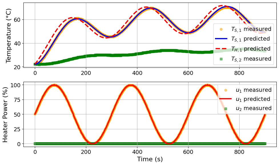
# visualize the SSE results
parmest_regression_results = extract_plot_results(
    tc_data, pest_SSE.ef_instance.exp_scenarios[0]
)

Model parameters:
Ua = 0.0417 Watts/°C
Ub = 0.0163 Watts/°C
CpH = 5.8757 Joules/°C
CpS = 0.3035 Joules/°C

Use the WSSE Objective to Estimate the Parameters¶

The WSSE objective falls naturally from the likelihood function of a Gaussian distribution that is not necessarily independent and identically distributed. In the WSSE, the difference between the model predictions and the data are scaled by the measurement error. For this reason, the WSSE serve as the most appropriate objective function for heterogeneous data with variables in different units of measure or magnitudes.

pest_WSSE = parmest.Estimator([TC_Lab_sine_exp], obj_function="SSE_weighted", tee=True)

obj_WSSE, theta_WSSE = pest_WSSE.theta_est()

Ipopt 3.13.2: 

******************************************************************************
This program contains Ipopt, a library for large-scale nonlinear optimization.
 Ipopt is released as open source code under the Eclipse Public License (EPL).
         For more information visit http://projects.coin-or.org/Ipopt

This version of Ipopt was compiled from source code available at
    https://github.com/IDAES/Ipopt as part of the Institute for the Design of
    Advanced Energy Systems Process Systems Engineering Framework (IDAES PSE
    Framework) Copyright (c) 2018-2019. See https://github.com/IDAES/idaes-pse.

This version of Ipopt was compiled using HSL, a collection of Fortran codes
    for large-scale scientific computation.  All technical papers, sales and
    publicity material resulting from use of the HSL codes within IPOPT must
    contain the following acknowledgement:
        HSL, a collection of Fortran codes for large-scale scientific
        computation. See http://www.hsl.rl.ac.uk.
******************************************************************************

This is Ipopt version 3.13.2, running with linear solver ma27.

Number of nonzeros in equality constraint Jacobian...:    15301
Number of nonzeros in inequality constraint Jacobian.:        0
Number of nonzeros in Lagrangian Hessian.............:     7203

Total number of variables............................:     3606
                     variables with only lower bounds:        0
                variables with lower and upper bounds:     1804
                     variables with only upper bounds:        0
Total number of equality constraints.................:     3602
Total number of inequality constraints...............:        0
        inequality constraints with only lower bounds:        0
   inequality constraints with lower and upper bounds:        0
        inequality constraints with only upper bounds:        0

iter    objective    inf_pr   inf_du lg(mu)  ||d||  lg(rg) alpha_du alpha_pr  ls
   0  3.7689956e+05 3.12e-01 1.00e+02  -1.0 0.00e+00    -  0.00e+00 0.00e+00   0
   1  6.9950237e+04 1.34e-01 6.09e+03  -1.0 1.00e+01    -  4.72e-01 5.76e-01f  1
   2  4.4812180e+02 2.63e-03 1.60e+03  -1.0 4.33e+00    -  9.31e-01 1.00e+00f  1
   3  4.3029017e+02 1.98e-05 8.77e+01  -1.0 5.40e-02    -  1.00e+00 1.00e+00f  1
   4  4.3019471e+02 6.02e-03 1.14e+01  -1.0 6.03e-01    -  1.00e+00 1.00e+00h  1
   5  4.3019369e+02 5.29e-03 9.95e-01  -1.0 4.64e-01    -  1.00e+00 1.00e+00h  1
   6  4.3019125e+02 1.21e-04 2.63e-02  -1.7 4.73e-02    -  1.00e+00 1.00e+00h  1
   7  4.3019194e+02 7.05e-08 2.41e-04  -3.8 1.18e-03    -  1.00e+00 1.00e+00h  1
   8  4.3019194e+02 7.86e-11 7.30e-06  -5.7 3.38e-03    -  1.00e+00 1.00e+00H  1
   9  4.3019194e+02 4.02e-11 6.20e-08  -8.6 3.67e-04    -  1.00e+00 1.00e+00H  1
iter    objective    inf_pr   inf_du lg(mu)  ||d||  lg(rg) alpha_du alpha_pr  ls
  10  4.3019194e+02 2.09e-03 3.35e-02  -8.6 2.69e-01    -  1.00e+00 1.00e+00h  1
  11  4.3019194e+02 2.09e-03 3.34e-02  -8.6 1.69e-02  -4.0 1.00e+00 4.88e-04h 12
  12  4.3019194e+02 2.09e-03 3.34e-02  -8.6 1.69e-02  -4.5 1.00e+00 3.05e-05h 16
  13  4.3019194e+02 2.09e-03 3.34e-02  -8.6 1.68e-02  -5.0 1.00e+00 1.53e-05h 17
  14  4.3019194e+02 2.09e-03 3.34e-02  -8.6 1.68e-02  -5.4 1.00e+00 1.53e-05h 17
  15  4.3019194e+02 2.09e-03 3.34e-02  -8.6 1.67e-02  -5.9 1.00e+00 1.53e-05h 17
  16  4.3019194e+02 1.51e-06 2.68e-05  -8.6 1.62e-02  -6.4 1.00e+00 1.00e+00h  1
  17  4.3019194e+02 2.25e-08 3.60e-07  -8.6 8.27e-04    -  1.00e+00 1.00e+00h  1
  18  4.3019194e+02 5.17e-08 8.27e-07  -8.6 1.24e-03    -  1.00e+00 1.00e+00h  1
  19  4.3019194e+02 1.01e-08 1.62e-07  -8.6 5.50e-04    -  1.00e+00 1.00e+00h  1
iter    objective    inf_pr   inf_du lg(mu)  ||d||  lg(rg) alpha_du alpha_pr  ls
  20  4.3019194e+02 5.27e-09 8.44e-08  -8.6 3.97e-04    -  1.00e+00 1.00e+00h  1
  21  4.3019194e+02 1.12e-08 1.79e-07  -8.6 5.78e-04    -  1.00e+00 1.00e+00h  1
  22  4.3019194e+02 5.60e-09 8.96e-08  -8.6 4.09e-04    -  1.00e+00 1.00e+00h  1
  23  4.3019194e+02 5.23e-09 8.36e-08  -8.6 5.39e-04    -  1.00e+00 5.00e-01h  2
  24  4.3019194e+02 7.67e-13 6.00e-10  -8.6 4.81e-06    -  1.00e+00 1.00e+00h  1

Number of Iterations....: 24

                                   (scaled)                 (unscaled)
Objective...............:   2.7451564684463716e+02    4.3019194276646789e+02
Dual infeasibility......:   5.9995251101476863e-10    9.4018224187830508e-10
Constraint violation....:   7.6694206541105814e-13    7.6694206541105814e-13
Complementarity.........:   2.5059035596800630e-09    3.9269875255390520e-09
Overall NLP error.......:   2.5059035596800630e-09    3.9269875255390520e-09


Number of objective function evaluations             = 104
Number of objective gradient evaluations             = 25
Number of equality constraint evaluations            = 104
Number of inequality constraint evaluations          = 0
Number of equality constraint Jacobian evaluations   = 25
Number of inequality constraint Jacobian evaluations = 0
Number of Lagrangian Hessian evaluations             = 24
Total CPU secs in IPOPT (w/o function evaluations)   =      0.134
Total CPU secs in NLP function evaluations           =      0.028

EXIT: Optimal Solution Found.

# visualize the WSSE results
WSSE_parmest_regression_results = extract_plot_results(
    tc_data, pest_WSSE.ef_instance.exp_scenarios[0]
)

Model parameters:
Ua = 0.0417 Watts/°C
Ub = 0.0171 Watts/°C
CpH = 5.8582 Joules/°C
CpS = 0.3187 Joules/°C

Compare the Parameter Estimates from SSE and WSSE¶

print("Model parameters using SSE objective:")
print("Ua =", round(theta_SSE["Ua"], 4), "Watts/°C")
print("Ub =", round(theta_SSE["Ub"], 4), "Watts/°C")
print("inv_CpH =", round(theta_SSE["inv_CpH"], 4), "°C/Joules")
print("inv_CpS =", round(theta_SSE["inv_CpS"], 4), "°C/Joules")

print("\nModel parameters using WSSE objective:")
print("Ua =", round(theta_WSSE["Ua"], 4), "Watts/°C")
print("Ub =", round(theta_WSSE["Ub"], 4), "Watts/°C")
print("inv_CpH =", round(theta_WSSE["inv_CpH"], 4), "°C/Joules")
print("inv_CpS =", round(theta_WSSE["inv_CpS"], 4), "°C/Joules")

Model parameters using SSE objective:
Ua = 0.0417 Watts/°C
Ub = 0.0163 Watts/°C
inv_CpH = 0.1702 °C/Joules
inv_CpS = 3.2951 °C/Joules

Model parameters using WSSE objective:
Ua = 0.0417 Watts/°C
Ub = 0.0171 Watts/°C
inv_CpH = 0.1707 °C/Joules
inv_CpS = 3.1379 °C/Joules

Activity: Try Different Measurement Errors¶

In this activity, you will explore how measurement error assumptions influence parameter estimation results using the WSSE objective.

# define the measurement errors in °C
meas_error = [0.1, 0.5, 1]

# define a list to store the result of the various measurement errors
activity_results_list = []

# for each of the measurement errors, estimate the parameters using ParmEst
for error in meas_error:
    # create a TC Lab experiment object
    exp = TC_Lab_experiment(
        data=tc_data, number_of_states=number_tclab_states, measurement_error=error
    )

    # create a ParmEst Estimator object
    pest = parmest.Estimator([exp], obj_function="SSE_weighted", tee=False)

    # estimate the parameters
    obj, theta_raw = pest.theta_est()
    theta = {
        "Ua (Watts/°C)": round(theta_raw["Ua"], 4),
        "Ub (Watts/°C)": round(theta_raw["Ub"], 4),
        "inv_CpH (°C/Joules)": round(theta_raw["inv_CpH"], 4),
        "inv_CpS (°C/Joules)": round(theta_raw["inv_CpS"], 4),
    }

    # add the measurement error associated with the parameter estimates
    theta["Measurement Error (°C)"] = error

    # update the list that stores the result of the various measurement errors
    activity_results_list.append(theta)

# store the activity results in a dataframe
activity_results_df = pd.DataFrame(activity_results_list).set_index(
    "Measurement Error (°C)"
)

# visualize the results
display(activity_results_df)

Takeaways from the Activity¶

Uniform measurement error has limited impact on parameter estimates
When the same measurement error is applied across all data points, the WSSE objective is rescaled, and the estimated parameters remain largely unchanged.
Small variations in the parameter estimates from SSE and WSSE (e.g., Ub and inv_CpS) can still occur from the choice of measurement error due to:
- Numerical solver tolerances
- Slight differences in convergence behavior
- Sensitivity of certain parameters to scaling