Exercise: ParmEst - Pyomo.DoE Workshop and Tutorials

In the main workshop tutorial, the four heat transfer parameters, $U_a$ , $U_b$ , $C_p^H$ , $C_p^S$ , were estimated from the sine test data using the following TC Lab model:

C_p^H \frac{dT_H}{dt} = U_a (T_{\text{amb}} - T_H) + U_b (T_S - T_H) + \alpha P u(t),

(1)

C_p^S \frac{dT_S}{dt} = U_b (T_H - T_S)

(2)

where $T_{H}$ and $T_{S}$ are the heater and sensor temperatures in $^{\circ} \text{C}$ , respectively, $T_{amb}$ is the ambient temperature in $^{\circ} \text{C}$ , $C_p^H$ and $C_p^S$ are the heat capacity of the heater and sensor in $\text{J}/^{\circ} \text{C}$ , respectively, $U_{a}$ and $U_{b}$ are the heat transfer coefficients from the heater to the sensor and the sensor to ambient (in $\text{W}/^{\circ} \text{C}$ ), respectively, $P$ is the maximum power limit in $\text{bit}$ , $u$ is the heater power in $\%$ , and $\alpha$ is constant that converts the unit of $P u(t)$ into $\text{W}$ .

As discussed in the uncertainty quantification section of the main workshop, the above model is structurally non-identifiable (i.e., the $U_a$ , $U_b$ , $C_p^H$ , and $C_p^S$ parameters cannot be reliably estimated from the mathematical structure of the model). To ensure accurate estimates of the model parameters, we need to explore other structures of the model that simplify parameter correlation.

In this exercise notebook, we present a reformulated, linearized (linear with respect to model parameters) version of the TC Lab model to reliably estimate the original parameters, $U_a$ , $U_b$ , $C_p^H$ , and $C_p^S$ from the sine test data. The structure of the reformulated model is:

\frac{dT_H}{dt} = \beta_1 (T_{\text{amb}} - T_H) + \beta_2 (T_S - T_H) + \beta_4 u(t),

(3)

\frac{dT_S}{dt} = \beta_3 (T_H - T_S)

(4)

where

\beta_1 = \frac{U_a}{C_p^H}, \quad \beta_2 = \frac{U_b}{C_p^H}, \quad \beta_3 = \frac{U_b}{C_p^S}, \quad \beta_4 = \frac{\alpha P}{C_p^H}

(5)

In this exercise, you will practice using ParmEst to estimate the reformulated model and then transform the estimates into the four original parameters ( $U_a$ , $U_b$ , $C_p^H$ , and $C_p^S$ ).

Implementing Reformulated Model in Pyomo¶

Take a few minutes to study the tclab_pyomo.py. Lines 420 to 520 (approximately) in file includes an implementation of the reformulated model. This file also supports regressing either the heat transfer coefficients, $U_a$ and $U_b$ , or their inverses, $1/U_a$ and $1/U_b$ , as model parameters.

Import the Necessary Packages for This Exercise¶

import sys
import numpy as np
import pandas as pd
import logging

# If running on Google Colab, install Pyomo and Ipopt via IDAES
on_colab = "google.colab" in sys.modules
if on_colab:
    !wget "https://raw.githubusercontent.com/dowlinglab/pyomo-doe/main/notebooks/tclab_pyomo.py"
else:
    import os

    if "exercise_solutions" in os.getcwd():
        # Add the "notebooks" folder to the path
        # This is needed for running the solutions from a separate folder
        # You only need this if you run locally
        sys.path.append("../notebooks")

# import TCLab model, simulation, and data analysis functions
from tclab_pyomo import (
    TC_Lab_data,
    TC_Lab_experiment,
    extract_results,
    extract_plot_results,
    plot_profile_likelihood,
    reformulate_parameters,
    recover_original_parameters,
    recover_original_covariance,
)

# set default number of states in the TCLab model
number_tclab_states = 2

Load and Explore Experimental Data (sine test)¶

if on_colab:
    file = "https://raw.githubusercontent.com/dowlinglab/pyomo-doe/main/data/tclab_sine_test_5min_period.csv"
else:
    file = "../data/tclab_sine_test_5min_period.csv"
df = pd.read_csv(file)
df[["Time", "T1", "Q1", "Q2"]].head()  # the Q2 column entries are 0 because
# we are considering the two-state model

Make two plots to visualize the temperature and heat power data as a function of time.

### BEGIN SOLUTION
ax = df.plot(x="Time", y=["T1"], xlabel="Time (s)", ylabel="Temperature (°C)")
### END SOLUTION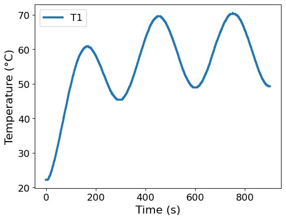

### BEGIN SOLUTION
ax = df.plot(x="Time", y=["Q1", "Q2"], xlabel="Time (s)", ylabel="Heater Power (%)")
### END SOLUTION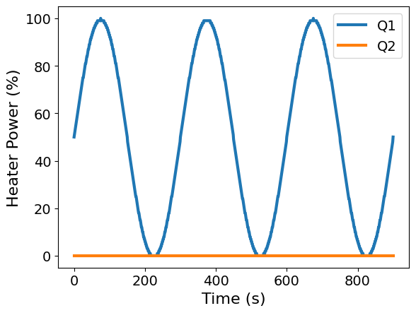

We’ll now store the data in this custom data class objective. This is a nice trick to help keep data organized, but it is NOT required to use ParmEst or Pyomo data. Alternatively, we could just use a pandas DataFrame.

tc_data = TC_Lab_data(
    name="Sine Wave Test for Heater 1",
    time=df["Time"].values,
    T1=df["T1"].values,
    u1=df["Q1"].values,
    P1=200,
    TS1_data=None,
    T2=df["T2"].values,
    u2=df["Q2"].values,
    P2=200,
    TS2_data=None,
    Tamb=df["T1"].values[0],
)

Our custom data class has a method to export the data as a Pandas Data Frame.

tc_data.to_data_frame().iloc[:, :4].head()

Parameter Estimation with ParmEst¶

Now for the main event: performing nonlinear least squares with ParmEst.

We seek to estimate the original parameters, $C_p^H$ , $C_p^S$ , $U_a$ , and $U_b$ from the reformulated TC Lab model (with $\beta_1$ , $\beta_2$ , $\beta_3$ , and $\beta_4$ as parameters) and the sensor data presented above.

The reformulated TC Lab model predicts the sensor data as follows:

\frac{dT_H}{dt} = \beta_1 (T_{\text{amb}} - T_H) + \beta_2 (T_S - T_H) + \beta_4 u(t),

(6)

\frac{dT_S}{dt} = \beta_3 (T_H - T_S)

(7)

\begin{align*} \text{control input data}\qquad u(t_i) & = \bar{u}_{i}, \forall i \in \mathcal{T} \\ \text{initial condition}\qquad T_H(t_0) & = T_{amb} \\ \text{initial condition}\qquad T_S(t_0) & = T_{amb} \end{align*}

(8)

Remember that

\beta_1 = \frac{U_a}{C_p^H}, \quad \beta_2 = \frac{U_b}{C_p^H}, \quad \beta_3 = \frac{U_b}{C_p^S}, \quad \beta_4 = \frac{\alpha P}{C_p^H}

(9)

In the tclab_pyomo.py model, we defined several helper functions:

extract_results takes a Pyomo model and returns the results stored in an instance of the TC_Lab_data dataclass.
extract_plot_results takes experimental data (stored in a TC_Lab_data instance) and a Pyomo model. The function then generates plots showing the data and model predictions.
results_summary summarizes the Pyomo.DoE results. We’ll use this later in the workshop.
reformulate_parameters reformulates the original parameters.
recover_original_parameters calculates the original parameters from the reformulated ones.
recover_original_covariance computes the covariance matrix of the original parameters from that of the reformulated parameters

import pyomo.contrib.parmest.parmest as parmest

# Set logging level to ERROR to suppress solver output and warnings from parmest
logging.basicConfig(level=logging.ERROR, force=True)

parmest_logger = logging.getLogger("pyomo.contrib.parmest.parmest")
parmest_logger.setLevel(logging.ERROR)

# Solver options used for all parmest estimation problems in this notebook
solver_options = {"linear_solver": "ma57", "max_iter": 1000, "max_cpu_time": 30}

# First, we define an Experiment object within parmest
#
# Hint: when calling TC_lab_experiment, set reparam=True to
# automatically reformulate the problem for better estimation performance
#
### BEGIN SOLUTION
TC_Lab_sine_exp = TC_Lab_experiment(
    data=tc_data, number_of_states=number_tclab_states, reparam=True
)
### END SOLUTION

# Since everything has been labeled properly in the Experiment object, we simply invoke
# parmest's Estimator function to estimate the parameters.
### BEGIN SOLUTION
pest = parmest.Estimator(
    [TC_Lab_sine_exp], obj_function="SSE", tee=True, solver_options=solver_options
)

obj, theta = pest.theta_est()
### END SOLUTION

Ipopt 3.13.2: linear_solver=ma57
max_iter=1000
max_cpu_time=30


******************************************************************************
This program contains Ipopt, a library for large-scale nonlinear optimization.
 Ipopt is released as open source code under the Eclipse Public License (EPL).
         For more information visit http://projects.coin-or.org/Ipopt

This version of Ipopt was compiled from source code available at
    https://github.com/IDAES/Ipopt as part of the Institute for the Design of
    Advanced Energy Systems Process Systems Engineering Framework (IDAES PSE
    Framework) Copyright (c) 2018-2019. See https://github.com/IDAES/idaes-pse.

This version of Ipopt was compiled using HSL, a collection of Fortran codes
    for large-scale scientific computation.  All technical papers, sales and
    publicity material resulting from use of the HSL codes within IPOPT must
    contain the following acknowledgement:
        HSL, a collection of Fortran codes for large-scale scientific
        computation. See http://www.hsl.rl.ac.uk.
******************************************************************************

This is Ipopt version 3.13.2, running with linear solver ma57.

Number of nonzeros in equality constraint Jacobian...:    14352
Number of nonzeros in inequality constraint Jacobian.:        0
Number of nonzeros in Lagrangian Hessian.............:     5400

Total number of variables............................:     3610
                     variables with only lower bounds:        0
                variables with lower and upper bounds:     1804
                     variables with only upper bounds:        0
Total number of equality constraints.................:     3606
Total number of inequality constraints...............:        0
        inequality constraints with only lower bounds:        0
   inequality constraints with lower and upper bounds:        0
        inequality constraints with only upper bounds:        0

iter    objective    inf_pr   inf_du lg(mu)  ||d||  lg(rg) alpha_du alpha_pr  ls
   0  4.7112445e+04 8.71e-01 1.12e+01  -1.0 0.00e+00    -  0.00e+00 0.00e+00   0
   1  4.3469867e+04 8.35e-01 8.12e+01  -1.0 1.15e+01    -  8.01e-01 4.14e-02f  1
   2  4.5250786e+01 4.53e-02 3.83e+03  -1.0 9.41e+00    -  8.72e-01 1.00e+00f  1
   3  5.6417595e+01 3.80e-03 1.56e+03  -1.0 7.50e-01    -  1.00e+00 1.00e+00h  1
   4  5.3783457e+01 1.00e-05 6.05e+00  -1.0 5.18e-02    -  1.00e+00 1.00e+00f  1
   5  5.3777952e+01 1.96e-03 5.12e-01  -1.0 4.74e-01    -  1.00e+00 1.00e+00f  1
   6  5.3773877e+01 2.59e-06 4.99e-02  -1.7 1.27e-02    -  1.00e+00 1.00e+00h  1
   7  5.3773998e+01 1.47e-06 1.25e-02  -2.5 1.37e-02    -  1.00e+00 1.00e+00h  1
   8  5.3773993e+01 1.72e-07 6.98e-04  -3.8 4.71e-03    -  1.00e+00 1.00e+00h  1
   9  5.3773993e+01 8.30e-09 8.96e-06  -5.7 1.04e-03    -  1.00e+00 1.00e+00h  1
iter    objective    inf_pr   inf_du lg(mu)  ||d||  lg(rg) alpha_du alpha_pr  ls
  10  5.3773993e+01 9.95e-11 1.15e-08  -8.6 1.15e-04    -  1.00e+00 1.00e+00h  1
  11  5.3773993e+01 2.45e-14 1.75e-09  -9.0 1.48e-08  -4.0 1.00e+00 1.00e+00h  1

Number of Iterations....: 11

                                   (scaled)                 (unscaled)
Objective...............:   5.3773992845808067e+01    5.3773992845808067e+01
Dual infeasibility......:   1.7516023792732849e-09    1.7516023792732849e-09
Constraint violation....:   2.4535928844215960e-14    2.4535928844215960e-14
Complementarity.........:   9.0909096874200624e-10    9.0909096874200624e-10
Overall NLP error.......:   1.7516023792732849e-09    1.7516023792732849e-09


Number of objective function evaluations             = 12
Number of objective gradient evaluations             = 12
Number of equality constraint evaluations            = 12
Number of inequality constraint evaluations          = 0
Number of equality constraint Jacobian evaluations   = 12
Number of inequality constraint Jacobian evaluations = 0
Number of Lagrangian Hessian evaluations             = 11
Total CPU secs in IPOPT (w/o function evaluations)   =      0.066
Total CPU secs in NLP function evaluations           =      0.008

EXIT: Optimal Solution Found.

parmest_regression_results = extract_plot_results(
    tc_data, pest.ef_instance.exp_scenarios[0], reparam=True
)

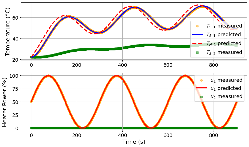
Model parameters:
Beta_1 = 0.0074 Watts/Joules
Beta_2 = 0.0048 Watts/Joules
Beta_3 = 0.0514 Watts/Joules
Beta_4 = 0.0057 °C.Watts/(Joules.%)

# Now that we have estimated the reformulated parameters, we
# need to transform them to the original parameters
theta_orig = recover_original_parameters(
    theta,
    alpha=pest.ef_instance.exp_scenarios[0].alpha,
    P1=pest.ef_instance.exp_scenarios[0].P1,
)

print("The original model parameters are:")
print("Ua =", round(theta_orig["Ua"], 4), "Watts/°C")
print("Ub =", round(theta_orig["Ub"], 4), "Watts/°C")
print("inv_CpH =", round(theta_orig["inv_CpH"], 4), "°C/Joules")
print("inv_CpS =", round(theta_orig["inv_CpS"], 4), "°C/Joules")

The original model parameters are:
Ua = 0.0417 Watts/°C
Ub = 0.0268 Watts/°C
inv_CpH = 0.1778 °C/Joules
inv_CpS = 1.9201 °C/Joules

Discussion: How do these results compare to our previous analysis? Discuss this in a few sentences.

Quantify the Uncertainty in the Parameter Estimates¶

As mentioned in the uncertainty quantification section of the main workshop, covariance matrix can be used to measure the accuracy of parameter estimates. This is needed to check how close the parameter estimates are to their true values. The leading diagonal of the covariance matrix contains the variance of the estimated parameters.

# Since everything has been labeled properly in the Experiment object, we
# simply use the `cov_est` function to compute the covariance matrix.
### BEGIN SOLUTION
cov = pest.cov_est(method="finite_difference")
### END SOLUTION

Fetching long content....

# Lets check the covariance matrix of the reformulated parameters
# Add a print statement to check the covariance matrix
### BEGIN SOLUTION
print("The covariance matrix of the reformulated parameters is:\n", cov)
### END SOLUTION

The covariance matrix of the reformulated parameters is:
              beta_1       beta_2       beta_3      beta_4
beta_1   168.950696  1002.082536 -1171.031849  129.634422
beta_2  1002.082536  5943.564807 -6945.639139  768.889347
beta_3 -1171.031849 -6945.639139  8116.661400 -898.522708
beta_4   129.634422   768.889347  -898.522708   99.467382

# since the covariance matrix is that of the reformulated parameters, we
# need to transform it to the original parameters
cov_orig = recover_original_covariance(
    theta,
    cov,
    alpha=pest.ef_instance.exp_scenarios[0].alpha,
    P1=pest.ef_instance.exp_scenarios[0].P1,
)

print("The covariance matrix of the original parameters is:\n", cov_orig)
print("\nThe trace of the covariance matrix is:", format(np.trace(cov_orig), ".3e"))

The covariance matrix of the original parameters is:
                    Ua            Ub       inv_CpH       inv_CpS
Ua       2.783708e-09 -1.970659e-02 -1.588585e-02  1.584949e+00
Ub      -1.970659e-02  1.494799e+05  1.204985e+05 -1.202228e+07
inv_CpH -1.588585e-02  1.204985e+05  9.713611e+04 -9.691381e+06
inv_CpS  1.584949e+00 -1.202228e+07 -9.691381e+06  9.669202e+08

The trace of the covariance matrix is: 9.672e+08

Discussion: How do these results compare to our previous analysis? Discuss this in a few sentences.

Multistart Optimization with ParmEst¶

Use multistart optimization with sobol sampling on the reformulated model.

pest_sobol = parmest.Estimator(
    [TC_Lab_sine_exp], obj_function="SSE", tee=True, solver_options=solver_options
)


# Set some common options for all multistart estimation runs
common_multistart_options = {"n_restarts": 15, "seed": 532, "save_results": False}

### BEGIN SOLUTION
results_df_sobol, best_theta_sobol, best_obj_sobol = pest_sobol.theta_est_multistart(
    multistart_sampling_method="sobol_sampling",
    n_restarts=common_multistart_options["n_restarts"],
    seed=common_multistart_options["seed"],
    save_results=common_multistart_options["save_results"],
)
### END SOLUTION

Fetching long content....

# Analyze results
print("Best parameter estimates from Sobol sampling multistart:")
print(best_theta_sobol)
print(f"Best objective value from Sobol sampling multistart: {best_obj_sobol}")

# Round the objective values to a reasonable number of decimal places for counting unique minima
results_df_sobol["final objective"] = results_df_sobol["final objective"].round(5)

num_unique_minima_sobol = len(results_df_sobol["final objective"].unique())
print(f"Number of unique minima found with Sobol sampling: {num_unique_minima_sobol}")

Best parameter estimates from Sobol sampling multistart:
{'beta_1': 0.007321147417889371, 'beta_2': 0.004188612160032208, 'beta_3': 0.05206952257325719, 'beta_4': 0.005617449791253524}
Best objective value from Sobol sampling multistart: 53.7739928458063
Number of unique minima found with Sobol sampling: 1

# Recalculate the original parameters from the best Sobol sampling result
orig_theta_sobol = recover_original_parameters(
    best_theta_sobol,
    alpha=pest.ef_instance.exp_scenarios[0].alpha,
    P1=pest.ef_instance.exp_scenarios[0].P1,
)

print("Estimated parameters:")
print(f"Ua: {orig_theta_sobol['Ua']:.6f} W/K")
print(f"Ub: {orig_theta_sobol['Ub']:.6f} W/K")
print(f"inv_CpH: {orig_theta_sobol['inv_CpH']:.6f} J/(K*kg)")
print(f"inv_CpS: {orig_theta_sobol['inv_CpS']:.6f} J/(K*kg)")

Estimated parameters:
Ua: 0.041705 W/K
Ub: 0.023861 W/K
inv_CpH: 0.175545 J/(K*kg)
inv_CpS: 2.182241 J/(K*kg)

Profile Likelihood with ParmEst¶

Analyze the profile likeihood of the reformulated model.

### BEGIN SOLUTION
profile_results = pest_sobol.profile_likelihood(
    profiled_theta=["beta_1", "beta_2", "beta_3", "beta_4"],
    obj_hat=best_obj_sobol,
    theta_hat=best_theta_sobol,
    n_grid=15,
    solver="ef_ipopt",
    warmstart="neighbor",
)
### END SOLUTION

Fetching long content....

profiles = profile_results["profiles"]
print("Profile likelihood results:")
profiles.head(5)

Profile likelihood results:

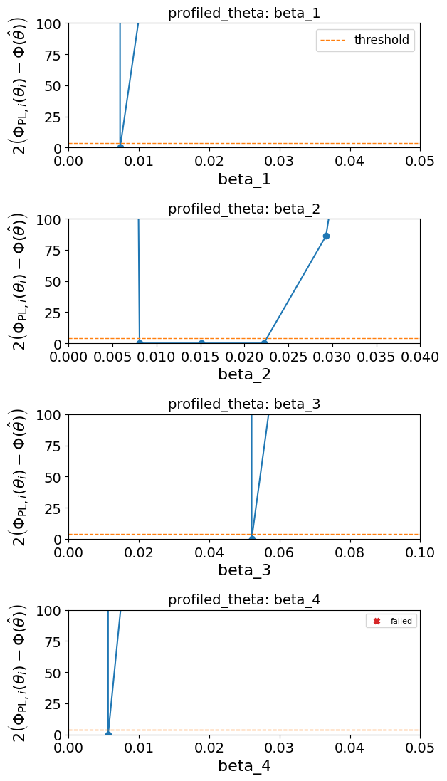
# Plot profile curves to visualize profile likelihood for each parameter.

### BEGIN SOLUTION
xlims = [(0, 0.05), (0, 0.04), (0, 0.1), (0, 0.05)]
ylims = [(0, 100), (0, 100), (0, 100), (0, 100)]

fig, axes = plot_profile_likelihood(
    profile_results, alpha=0.95, xlims=xlims, ylims=ylims
)
### END SOLUTION

Chi-squared threshold for 95% confidence interval: 3.8415

How does the estimability of the reformulated model compare to the original model?

Add L2 Regularization to Parameter Estimation Objective¶

Using the same prior from the regularization notebook, converted to the reformulated model parameters, add regularization and compare the optimal solution.

# Original prior:

# ---- Physically intuitive guesses (Cp-space) ----
theta_phys = pd.Series(
    {"Ua": 0.030, "Ub": 0.018, "inv_CpH": 1 / 7.5, "inv_CpS": 1 / 0.22}
)


# Transform to estimator parameterization [beta-space]
theta0_phys_reparam = reformulate_parameters(
    theta_phys,
    alpha=pest.ef_instance.exp_scenarios[0].alpha,
    P1=pest.ef_instance.exp_scenarios[0].P1,
)

# Define diagonal covariance matrix
cov_x = pd.DataFrame(
    np.diag([0.02, 0.01, 0.05, 0.05]),
    index=["beta_1", "beta_2", "beta_3", "beta_4"],
    columns=["beta_1", "beta_2", "beta_3", "beta_4"],
)

# Invert to get the physically informed prior_FIM
prior_FIM_phys = pd.DataFrame(
    np.linalg.inv(cov_x.values), index=cov_x.index, columns=cov_x.columns
)

# Optional scaling factor to tune regularization strength
prior_weight = 2
prior_FIM_phys = prior_weight * prior_FIM_phys


print("theta0_phys_reparam:", theta0_phys_reparam)
print("prior_FIM_phys:\n", prior_FIM_phys)

theta0_phys_reparam: {'beta_1': np.float64(0.004), 'beta_2': np.float64(0.0024), 'beta_3': np.float64(0.08181818181818182), 'beta_4': np.float64(0.004266666666666667)}
prior_FIM_phys:
         beta_1  beta_2  beta_3  beta_4
beta_1   100.0     0.0     0.0     0.0
beta_2     0.0   200.0     0.0     0.0
beta_3     0.0     0.0    40.0     0.0
beta_4     0.0     0.0     0.0    40.0

### BEGIN SOLUTION
pest_regL2 = parmest.Estimator(
    [TC_Lab_sine_exp],
    obj_function="SSE_weighted",
    tee=True,
    solver_options=solver_options,
    regularization="L2",
    prior_FIM=prior_FIM_phys,
    theta_ref=theta0_phys_reparam,
)

obj_phys, theta_phys_est = pest_regL2.theta_est()

print("\nL2 (physical prior) objective:", obj_phys)
print("L2 (physical prior) theta:\n", theta_phys_est)
### END SOLUTION

Ipopt 3.13.2: linear_solver=ma57
max_iter=1000
max_cpu_time=30


******************************************************************************
This program contains Ipopt, a library for large-scale nonlinear optimization.
 Ipopt is released as open source code under the Eclipse Public License (EPL).
         For more information visit http://projects.coin-or.org/Ipopt

This version of Ipopt was compiled from source code available at
    https://github.com/IDAES/Ipopt as part of the Institute for the Design of
    Advanced Energy Systems Process Systems Engineering Framework (IDAES PSE
    Framework) Copyright (c) 2018-2019. See https://github.com/IDAES/idaes-pse.

This version of Ipopt was compiled using HSL, a collection of Fortran codes
    for large-scale scientific computation.  All technical papers, sales and
    publicity material resulting from use of the HSL codes within IPOPT must
    contain the following acknowledgement:
        HSL, a collection of Fortran codes for large-scale scientific
        computation. See http://www.hsl.rl.ac.uk.
******************************************************************************

This is Ipopt version 3.13.2, running with linear solver ma57.

Number of nonzeros in equality constraint Jacobian...:    14352
Number of nonzeros in inequality constraint Jacobian.:        0
Number of nonzeros in Lagrangian Hessian.............:     5404

Total number of variables............................:     3610
                     variables with only lower bounds:        0
                variables with lower and upper bounds:     1804
                     variables with only upper bounds:        0
Total number of equality constraints.................:     3606
Total number of inequality constraints...............:        0
        inequality constraints with only lower bounds:        0
   inequality constraints with lower and upper bounds:        0
        inequality constraints with only upper bounds:        0

iter    objective    inf_pr   inf_du lg(mu)  ||d||  lg(rg) alpha_du alpha_pr  ls
   0  6.0226828e+06 3.89e+01 5.48e+01  -1.0 0.00e+00    -  0.00e+00 0.00e+00   0
   1  5.9617972e+06 3.82e+01 2.60e+02  -1.0 2.67e+02   0.0 7.57e-03 1.65e-02f  1
   2  5.9613033e+06 3.82e+01 1.75e+02  -1.0 2.84e+01   0.4 9.78e-02 4.79e-04f  1
   3  5.5219428e+06 1.14e+01 3.40e+04  -1.0 2.33e+01   0.9 7.10e-02 9.75e-01f  1
   4  5.1326802e+06 1.09e+01 3.39e+04  -1.0 7.18e+01    -  3.82e-02 4.04e-02f  1
   5  3.1032281e+06 8.40e+00 2.93e+04  -1.0 9.02e+01    -  7.68e-02 2.32e-01f  1
   6  3.1061235e+06 8.37e+00 2.93e+04  -1.0 4.08e+01   0.4 2.08e-02 3.59e-03h  1
   7  3.3463238e+06 8.07e+00 1.10e+05  -1.0 5.63e+01  -0.1 2.04e-01 3.61e-02h  4
   8  2.9149357e+06 7.47e+00 4.34e+05  -1.0 4.12e+01   0.3 1.27e-01 7.40e-02f  1
   9  2.8170898e+06 6.55e+00 4.11e+05  -1.0 1.25e+02    -  1.05e-01 1.22e-01H  1
iter    objective    inf_pr   inf_du lg(mu)  ||d||  lg(rg) alpha_du alpha_pr  ls
  10  2.2894913e+06 4.98e+00 9.98e+06  -1.0 4.04e+01   1.7 1.28e-02 2.39e-01f  1
  11  2.2890911e+06 4.98e+00 9.97e+06  -1.0 2.89e+01   1.2 2.11e-01 1.08e-03f  1
  12  2.2866409e+06 4.97e+00 9.95e+06  -1.0 2.99e+01   1.6 5.55e-02 2.28e-03f  1
  13  2.2840318e+06 4.95e+00 9.92e+06  -1.0 2.98e+01   1.1 6.68e-03 2.83e-03f  1
  14  2.1861252e+06 4.57e+00 9.35e+06  -1.0 3.01e+01   1.6 4.37e-03 7.81e-02f  1
  15  2.1861352e+06 4.56e+00 9.75e+06  -1.0 3.42e+01   1.1 1.06e-01 1.33e-05h  1
  16  2.1862880e+06 4.56e+00 9.76e+06  -1.0 2.82e+01   0.6 1.01e-03 5.34e-04h  1
  17  2.1828390e+06 4.52e+00 9.58e+06  -1.0 2.65e+01   1.0 5.47e-05 1.00e-02f  1
  18  2.1133256e+06 4.12e+00 8.73e+06  -1.0 2.68e+01   1.4 7.54e-02 8.75e-02f  1
  19  2.1134362e+06 4.12e+00 9.12e+06  -1.0 2.46e+01   1.0 5.08e-02 3.94e-04h  1
iter    objective    inf_pr   inf_du lg(mu)  ||d||  lg(rg) alpha_du alpha_pr  ls
  20  2.1130760e+06 4.10e+00 9.03e+06  -1.0 2.43e+01    -  1.77e-03 4.19e-03f  1
  21  2.0513463e+06 3.57e+00 7.80e+06  -1.0 2.36e+01   1.4 8.38e-05 1.30e-01f  1
  22  2.0516628e+06 3.57e+00 8.25e+06  -1.0 2.15e+01   0.9 9.77e-02 4.22e-04h  1
  23  2.0494300e+06 3.53e+00 8.10e+06  -1.0 1.99e+01    -  2.28e-03 9.25e-03f  1
  24  2.0434808e+06 3.45e+00 7.89e+06  -1.0 1.95e+01   1.3 9.68e-05 2.43e-02f  1
  25  2.0434650e+06 3.45e+00 7.94e+06  -1.0 1.85e+01   0.9 8.39e-03 2.64e-04f  1
  26  2.0340830e+06 3.35e+00 7.49e+06  -1.0 1.91e+01    -  1.27e-04 2.89e-02f  1
  27  2.0120000e+06 2.83e+00 6.37e+06  -1.0 1.82e+01   1.3 1.51e-01 1.54e-01f  1
  28  2.0124909e+06 2.83e+00 6.35e+06  -1.0 1.80e+01   0.8 9.52e-02 4.08e-04h  1
  29  1.9953457e+06 2.72e+00 6.07e+06  -1.0 1.54e+01    -  3.04e-04 4.06e-02f  1
iter    objective    inf_pr   inf_du lg(mu)  ||d||  lg(rg) alpha_du alpha_pr  ls
  30  1.9875344e+06 2.19e+00 5.23e+06  -1.0 1.41e+01   1.2 3.40e-02 1.95e-01f  1
  31  1.9880532e+06 2.19e+00 4.96e+06  -1.0 1.19e+01   0.8 1.12e-01 6.61e-04h  1
  32  1.8494411e+06 1.35e+00 4.13e+06  -1.0 1.19e+01    -  1.35e-03 3.84e-01f  1
  33  1.8327773e+06 5.65e-01 1.76e+06  -1.0 6.68e+00   1.2 6.16e-01 5.80e-01f  1
  34  1.7909753e+06 3.94e-01 1.65e+06  -1.0 3.24e+00   0.7 3.13e-02 3.02e-01f  1
  35  1.7885098e+06 3.93e-01 1.63e+06  -1.0 1.11e+01   0.2 1.35e-02 2.77e-03f  1
  36  1.7885041e+06 3.93e-01 1.63e+06  -1.0 2.64e+00   0.7 4.41e-03 4.74e-05h  1
  37  1.7026134e+06 3.66e-01 1.60e+06  -1.0 1.64e+01   0.2 2.90e-04 6.83e-02f  1
  38  1.7007581e+06 3.62e-01 7.19e+05  -1.0 2.51e+00   0.6 5.90e-01 1.07e-02f  1
  39  1.7001481e+06 3.61e-01 7.18e+05  -1.0 3.59e+00    -  7.20e-04 2.97e-03f  1
iter    objective    inf_pr   inf_du lg(mu)  ||d||  lg(rg) alpha_du alpha_pr  ls
  40  1.6038746e+06 3.26e-01 6.99e+05  -1.0 1.29e+01   0.1 5.07e-05 9.93e-02f  1
  41  1.6019103e+06 3.22e-01 6.09e+05  -1.0 2.51e+00   0.6 1.46e-01 1.10e-02f  1
  42  1.5898879e+06 3.17e-01 6.07e+05  -1.0 9.77e+00   0.1 1.21e-04 1.65e-02f  1
  43  1.4523456e+06 8.88e-02 4.78e+05  -1.0 2.84e+00   0.5 4.11e-02 7.21e-01f  1
  44  1.2174126e+06 6.55e-01 5.13e+05  -1.0 8.18e+00   0.0 1.81e-03 4.69e-01f  1
  45  1.2423204e+06 6.23e-01 5.02e+05  -1.0 4.42e+00   0.5 8.90e-03 2.89e-02H  1
  46  8.1038734e+05 3.34e-01 9.06e+05  -1.0 8.48e+00  -0.0 3.56e-04 5.83e-01f  1
  47  2.5818917e+05 2.04e-01 7.38e+05  -1.0 1.94e+01    -  3.87e-04 1.00e+00f  1
  48  4.7578956e+03 3.40e-02 3.17e+05  -1.0 1.18e+01    -  5.38e-01 1.00e+00f  1
  49  5.3461430e+02 9.90e-03 2.35e+04  -1.0 1.72e+00    -  9.06e-01 1.00e+00f  1
iter    objective    inf_pr   inf_du lg(mu)  ||d||  lg(rg) alpha_du alpha_pr  ls
  50  4.3124046e+02 2.00e-04 2.34e+02  -1.0 1.71e-01    -  9.91e-01 1.00e+00f  1
  51  4.3047009e+02 3.12e-05 5.00e-01  -1.0 5.95e-02    -  1.00e+00 1.00e+00f  1
  52  4.3021726e+02 7.91e-05 4.56e-01  -1.7 9.76e-02    -  1.00e+00 1.00e+00h  1
  53  4.3022086e+02 6.01e-04 9.15e-03  -1.7 2.67e-01    -  1.00e+00 1.00e+00h  1
  54  4.3020987e+02 3.19e-07 9.95e-03  -3.8 7.21e-03    -  1.00e+00 1.00e+00h  1
  55  4.3020818e+02 3.21e-04 4.36e-04  -3.8 2.03e-01    -  1.00e+00 1.00e+00h  1
  56  4.3020704e+02 1.18e-04 8.80e-04  -5.7 1.17e-01    -  9.93e-01 1.00e+00h  1
  57  4.3020629e+02 7.29e-05 3.97e-05  -5.7 9.11e-02    -  1.00e+00 1.00e+00h  1
  58  4.3020620e+02 1.15e-06 6.23e-07  -5.7 1.07e-02    -  1.00e+00 1.00e+00h  1
  59  4.3020616e+02 1.96e-07 5.13e-07  -8.6 4.69e-03    -  1.00e+00 1.00e+00h  1
iter    objective    inf_pr   inf_du lg(mu)  ||d||  lg(rg) alpha_du alpha_pr  ls
  60  4.3020616e+02 6.50e-11 3.98e-10  -8.6 8.38e-05    -  1.00e+00 1.00e+00h  1

Number of Iterations....: 60

                                   (scaled)                 (unscaled)
Objective...............:   2.3432855542453503e+01    4.3020616217133528e+02
Dual infeasibility......:   3.9804211158706563e-10    7.3076953382061627e-09
Constraint violation....:   6.4999505777763034e-11    6.4999672311216727e-11
Complementarity.........:   2.5117022202493919e-09    4.6112594802330923e-08
Overall NLP error.......:   2.5117022202493919e-09    4.6112594802330923e-08


Number of objective function evaluations             = 68
Number of objective gradient evaluations             = 61
Number of equality constraint evaluations            = 68
Number of inequality constraint evaluations          = 0
Number of equality constraint Jacobian evaluations   = 61
Number of inequality constraint Jacobian evaluations = 0
Number of Lagrangian Hessian evaluations             = 60
Total CPU secs in IPOPT (w/o function evaluations)   =      0.428
Total CPU secs in NLP function evaluations           =      0.060

EXIT: Optimal Solution Found.

L2 (physical prior) objective: 430.2061621713352
L2 (physical prior) theta:
 beta_1    0.006839
beta_2    0.001000
beta_3    0.055740
beta_4    0.005248
dtype: float64

# Compare to unregularized estimation results and multistart results
print("\nUnregularized objective:", obj)
print("Unregularized theta:\n", theta)

print("\nBest Sobol multistart objective:", best_obj_sobol)
print(
    "Best Sobol multistart theta:\n",
    pd.DataFrame(best_theta_sobol, index=["best_theta"]).T,
)

print("\nL2 (physical prior) objective:", obj_phys)
print("L2 (physical prior) theta:\n", theta_phys_est)


Unregularized objective: 53.77399284580807
Unregularized theta:
 beta_1    0.007416
beta_2    0.004760
beta_3    0.051403
beta_4    0.005690
dtype: float64

Best Sobol multistart objective: 53.7739928458063
Best Sobol multistart theta:
         best_theta
beta_1    0.007321
beta_2    0.004189
beta_3    0.052070
beta_4    0.005617

L2 (physical prior) objective: 430.2061621713352
L2 (physical prior) theta:
 beta_1    0.006839
beta_2    0.001000
beta_3    0.055740
beta_4    0.005248
dtype: float64