Parameter estimation problems can be challenging when the available data are limited, noisy, or weakly informative for some parameters. In these cases, the least squares or maximum likelihood objective may have broad valleys, multiple local optima, or parameter estimates that are physically unreasonable.
One way to incorporate additional information is through regularization. Regularization augments the parameter estimation objective with an additional term that penalizes deviations from prior parameter values.
Let denote a vector of prior or nominal parameter values, and let denote a prior Fisher information matrix (FIM). The prior FIM represents the amount of information available about the parameters before fitting the current data. This information may come from previous experiments, previous parameter estimation studies, literature values, or expert knowledge.
The regularized parameter estimation problem can be written as
where is the objective function from the current parameter estimation problem and is the regularization term.
Maximum Likelihood Estimation and Regularization
The current ParmEst parameter estimation workflow can be interpreted as a
maximum likelihood estimation (MLE) problem when the objective function is
derived from an assumed measurement error distribution.
For example, when Gaussian independent measurement errors are assumed, the weighted sum of squared errors objective corresponds to the negative log-likelihood of the observed data, up to additive constants. In this case, solving
is equivalent to finding the maximum likelihood estimate:
or, equivalently,
Regularization modifies this objective by adding prior information about the parameters. The regularized problem is
This can be viewed as a bridge between MLE and Bayesian parameter estimation.
Import the Necessary Packages
import sys
import numpy as np
import pandas as pd

# If running on Google Colab, install Pyomo and Ipopt via IDAES
on_colab = "google.colab" in sys.modules
if on_colab:
    !wget "https://raw.githubusercontent.com/dowlinglab/pyomo-doe/main/notebooks/tclab_pyomo.py"

# import TCLab model, simulation, and data analysis functions
from tclab_pyomo import TC_Lab_data, TC_Lab_experiment

# set default number of states in the TCLab model
number_tclab_states = 2
Load Experimental Data
# load experimental data
if on_colab:
    file = "https://raw.githubusercontent.com/dowlinglab/pyomo-doe/main/data/tclab_sine_test_5min_period.csv"
else:
    file = "../data/tclab_sine_test_5min_period.csv"
df = pd.read_csv(file)

# store in custom data class
tc_data = TC_Lab_data(
    name="Sine Wave Test for Heater 1",
    time=df["Time"].values,
    T1=df["T1"].values,
    u1=df["Q1"].values,
    P1=200,
    TS1_data=None,
    T2=df["T2"].values,
    u2=df["Q2"].values,
    P2=200,
    TS2_data=None,
    Tamb=df["T1"].values[0],
)

# set default number of states in the TCLab model
number_tclab_states = 2
Interpretation of the Prior FIM
The prior FIM provides a way to encode prior information in a form that is consistent with the local curvature of a parameter estimation objective.
A larger value in indicates that the prior information strongly constrains a parameter or parameter combination. A smaller value indicates weaker prior information. If the prior FIM contains off-diagonal terms, then the regularization accounts for correlations between parameter directions.
For regularization, the full prior FIM can be used directly:
Physically Motivated Prior Information
For regularization, we define a weakly informative prior using physical intuition, literature values, and expert knowledge. The purpose of this prior is not to fix the parameter estimates, but to guide the optimization toward physically reasonable values when the data are not strongly informative.
The nominal physical parameter values are
Here, represents heat loss from the heater to the surroundings, represents heater-to-sensor coupling, is the heater thermal mass, and is the sensor thermal mass. These values reflect the expectation that the heater has a much larger effective heat capacity than the sensor, while both thermal conductance parameters are small but nonzero.
Because the estimator uses inverse heat capacities, the prior is transformed to
To represent uncertainty in this prior, we specify a diagonal covariance matrix in the estimator parameterization:
The diagonal form assumes no prior correlations, and the relatively large variances make the prior weakly informative. The prior Fisher information matrix is then computed as
This scaled prior FIM is used in the regularization term to discourage physically unrealistic parameter values while still allowing the experimental data to dominate the estimate.
# Regularization using physically informed prior

# ---- Physically intuitive guesses (Cp-space) ----
theta_phys = pd.Series(
    {
        "Ua": 0.030,  # W/K, ambient loss from heater node
        "Ub": 0.018,  # W/K, heater-to-sensor coupling
        "CpH": 7.5,  # J/K, heater thermal mass
        "CpS": 0.22,  # J/K, sensor thermal mass
    }
)


# Transform to estimator parameterization [Ua, Ub, inv_CpH, inv_CpS]
theta0_phys = pd.Series(
    {
        "Ua": theta_phys["Ua"],
        "Ub": theta_phys["Ub"],
        "inv_CpH": 1.0 / theta_phys["CpH"],
        "inv_CpS": 1.0 / theta_phys["CpS"],
    }
)

# Define diagonal covariance matrix
cov_x = pd.DataFrame(
    np.diag([0.02, 0.01, 0.05, 0.05]),
    index=["Ua", "Ub", "inv_CpH", "inv_CpS"],
    columns=["Ua", "Ub", "inv_CpH", "inv_CpS"],
)

# Invert to get the physically informed prior_FIM
prior_FIM_phys = pd.DataFrame(
    np.linalg.inv(cov_x.values), index=cov_x.index, columns=cov_x.columns
)

# Optional scaling factor to tune regularization strength
prior_weight = 2
prior_FIM_phys = prior_weight * prior_FIM_phys


print("theta0_phys:", theta0_phys)
print("prior_FIM_phys:\n", prior_FIM_phys)
theta0_phys: Ua 0.030000
Ub 0.018000
inv_CpH 0.133333
inv_CpS 4.545455
dtype: float64
prior_FIM_phys:
Ua Ub inv_CpH inv_CpS
Ua 100.0 0.0 0.0 0.0
Ub 0.0 200.0 0.0 0.0
inv_CpH 0.0 0.0 40.0 0.0
inv_CpS 0.0 0.0 0.0 40.0
Adding Regularization to Objective in ParmEst
In regularization, the penalty is quadratic in the difference between the estimated parameters and the prior parameter values.
Using a prior FIM, the regularization term can be written as
so that the regularized parameter estimation problem becomes
This term penalizes parameter values that move far away from the prior values. The prior FIM determines both the magnitude and correlation structure of the penalty. Parameters with larger prior information are penalized more strongly for moving away from their prior values, while correlations in the prior FIM allow coupled parameter deviations to be represented.
regularization is smooth and differentiable, which makes it convenient for gradient-based nonlinear optimization solvers.
# # Import parmest
import pyomo.contrib.parmest.parmest as parmest
# Define an Experiment object within parmest
TC_Lab_sine_exp = TC_Lab_experiment(data=tc_data, number_of_states=number_tclab_states)
solver_options = {"linear_solver": "ma57"}
# Since everything has been labeled properly in the Experiment object, we simply invoke
# parmest's Estimator function to estimate the parameters and add the needed regularization arguments.
pest_regL2_phys = parmest.Estimator(
[TC_Lab_sine_exp],
obj_function="SSE_weighted",
tee=True,
solver_options=solver_options,
regularization="L2",
prior_FIM=prior_FIM_phys,
theta_ref=theta0_phys,
)
obj_phys, theta_phys_est = pest_regL2_phys.theta_est()
print("\nL2 (physical prior) objective:", obj_phys)
print("L2 (physical prior) theta:\n", theta_phys_est)Ipopt 3.13.2: linear_solver=ma57
******************************************************************************
This program contains Ipopt, a library for large-scale nonlinear optimization.
Ipopt is released as open source code under the Eclipse Public License (EPL).
For more information visit http://projects.coin-or.org/Ipopt
This version of Ipopt was compiled from source code available at
https://github.com/IDAES/Ipopt as part of the Institute for the Design of
Advanced Energy Systems Process Systems Engineering Framework (IDAES PSE
Framework) Copyright (c) 2018-2019. See https://github.com/IDAES/idaes-pse.
This version of Ipopt was compiled using HSL, a collection of Fortran codes
for large-scale scientific computation. All technical papers, sales and
publicity material resulting from use of the HSL codes within IPOPT must
contain the following acknowledgement:
HSL, a collection of Fortran codes for large-scale scientific
computation. See http://www.hsl.rl.ac.uk.
******************************************************************************
This is Ipopt version 3.13.2, running with linear solver ma57.
Number of nonzeros in equality constraint Jacobian...: 15309
Number of nonzeros in inequality constraint Jacobian.: 0
Number of nonzeros in Lagrangian Hessian.............: 7207
Total number of variables............................: 3610
variables with only lower bounds: 0
variables with lower and upper bounds: 1804
variables with only upper bounds: 0
Total number of equality constraints.................: 3606
Total number of inequality constraints...............: 0
inequality constraints with only lower bounds: 0
inequality constraints with lower and upper bounds: 0
inequality constraints with only upper bounds: 0
iter objective inf_pr inf_du lg(mu) ||d|| lg(rg) alpha_du alpha_pr ls
0 3.7693883e+05 3.12e-01 1.00e+02 -1.0 0.00e+00 - 0.00e+00 0.00e+00 0
1 4.4870961e+02 3.25e-02 1.83e+04 -1.0 1.00e+01 - 6.11e-01 1.00e+00f 1
2 4.2698049e+02 9.30e-04 1.57e+02 -1.0 2.27e-01 - 9.91e-01 1.00e+00f 1
3 4.3020268e+02 1.26e-04 1.56e+00 -1.0 9.64e-02 - 1.00e+00 1.00e+00h 1
4 4.3022778e+02 1.16e-08 2.71e-04 -1.0 7.15e-04 - 1.00e+00 1.00e+00h 1
5 4.3022567e+02 2.45e-07 3.39e-02 -2.5 3.72e-03 - 1.00e+00 1.00e+00h 1
6 4.3022567e+02 5.05e-12 8.28e-07 -2.5 1.91e-05 - 1.00e+00 1.00e+00h 1
7 4.3022567e+02 1.89e-10 2.63e-05 -3.8 1.04e-04 - 1.00e+00 1.00e+00h 1
8 4.3022567e+02 5.86e-13 8.13e-08 -5.7 5.76e-06 - 1.00e+00 1.00e+00h 1
9 4.3022567e+02 2.60e-14 5.01e-10 -8.6 7.13e-08 - 1.00e+00 1.00e+00h 1
Number of Iterations....: 9
(scaled) (unscaled)
Objective...............: 2.7453716992070184e+02 4.3022567136969508e+02
Dual infeasibility......: 5.0117495257881927e-10 7.8538847948777747e-10
Constraint violation....: 2.5951463200613034e-14 2.5951463200613034e-14
Complementarity.........: 2.5060833993855206e-09 3.9272693505236773e-09
Overall NLP error.......: 2.5060833993855206e-09 3.9272693505236773e-09
Number of objective function evaluations = 10
Number of objective gradient evaluations = 10
Number of equality constraint evaluations = 10
Number of inequality constraint evaluations = 0
Number of equality constraint Jacobian evaluations = 10
Number of inequality constraint Jacobian evaluations = 0
Number of Lagrangian Hessian evaluations = 9
Total CPU secs in IPOPT (w/o function evaluations) = 0.054
Total CPU secs in NLP function evaluations = 0.015
EXIT: Optimal Solution Found.
L2 (physical prior) objective: 430.2256713696951
L2 (physical prior) theta:
Ua 0.041705
Ub 0.012009
inv_CpH 0.167457
inv_CpS 4.545432
dtype: float64
# Calculate covariance of parameter estimates for regularized estimation with physical prior
cov_regL2_phys = pest_regL2_phys.cov_est()
print(
    "\nCovariance of parameter estimates with L2 regularization and physical prior:\n",
    cov_regL2_phys,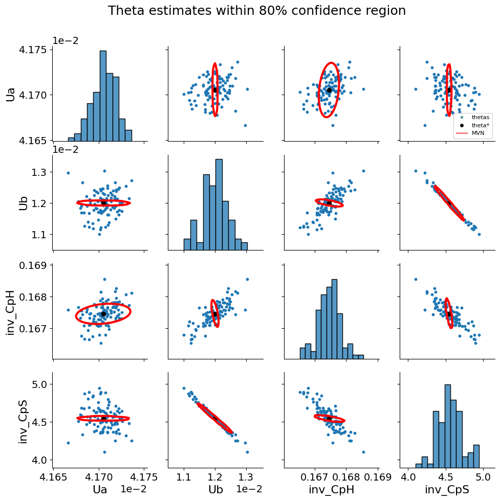
)We can view the confidence intervals of the estimated parameters using the regularized objective with the implmmented tool below.
if parmest.graphics.seaborn_available:
    parmest.graphics.pairwise_plot(
        (theta_phys_est, cov_regL2_phys, 100),
        theta_star=theta_phys_est,
        alpha=0.8,
        distributions=["MVN"],
        title="Theta estimates within 80% confidence region",
    )
Connection to MAP Estimation
Maximum a posteriori (MAP) estimation incorporates both the likelihood of the data and a prior distribution over the parameters. The MAP estimate is defined as
Using Bayes’ rule,
so that MAP estimation can be written as
The first term corresponds to the parameter estimation objective from the current data. The second term corresponds to a regularization term induced by the prior distribution.
For example, an regularization term corresponds to a Gaussian prior centered at :
The negative log-prior is proportional to
which is the regularization term.
Activity: How Does the Strength of the Prior Affect the Parameter Estimation?
How does the strength of the physical prior affect the estimate covariance, and the Fisher information matrix of the system?
One goal of using regularization is to improve the conditioning of the covariance results. Another way to say this is regularization raises the minimum eigenvalue of the Fisher information matrix, improving the overall estimability.
In the cell below, the main control is a variable, prior_weight which is previously set to 2. How does adjusting the prior weight impact the results?
# Redefine the prior_FIM_phys with a scaling factor to demonstrate tuning regularization strength
prior_FIM_phys = pd.DataFrame(
    np.linalg.inv(cov_x.values), index=cov_x.index, columns=cov_x.columns
)


# Helper to compute metrics from a covariance matrix (accepts pandas DataFrame or ndarray)
def cov_metrics(cov):
    cov_arr = cov.values if hasattr(cov, "values") else np.asarray(cov)
    FIM = np.linalg.inv(cov_arr)
    eigs = np.linalg.eigvals(FIM)
    return {
        "trace_cov": np.trace(cov_arr),
        "determinant_FIM": np.linalg.det(FIM),
        "min_eigenvalue_FIM": np.min(eigs).real,
        "condition_number_FIM": np.linalg.cond(FIM),
    }


# Ensure original covariance exists (from prior_weight=2 run)
cov_orig = cov_regL2_phys

metrics_orig = cov_metrics(cov_orig)
# Choose a new prior weight to demonstrate the effect of tuning regularization strength
prior_weight = 1
prior_FIM_activity = prior_weight * prior_FIM_phys
# Calculate the parameter estimates with the new scaled prior_FIM_phys to demonstrate tuning regularization strength
pest_activity = parmest.Estimator(
[TC_Lab_sine_exp],
obj_function="SSE_weighted",
solver_options=solver_options,
regularization="L2",
prior_FIM=prior_FIM_activity,
theta_ref=theta0_phys,
)
obj_activity, theta_activity = pest_activity.theta_est()
# Calculate covariance of parameter estimates for regularized estimation with physical prior
cov_activity = pest_activity.cov_est()
metrics_current = cov_metrics(cov_activity)
# Assemble comparison table
orig_col = "prior_weight=2 (original)"
cur_col = f"prior_weight={prior_weight} (current)"
comparison = pd.DataFrame({orig_col: metrics_orig, cur_col: metrics_current})
# display the table
comparison = comparison.T
comparison.round(6)Takeaways from the Activity
Increasing the strength of the prior reduces the uncertainty.
Use caution when doing this from physical intuition unless confident in the results.
This FIM activity is a simple example of what is done with design of experiments in Pyomo.DoE next session to pick experimental conditions.